When simulating random variables in statistics or machine learning, we often need samples from a standard normal distribution. However, programming languages that are not focused on statistics often lack a rich suite of random number generators for various distributions. Therefore, it is essential to know how to implement such generators from scratch, typically using uniformly distributed pseudo-random numbers. This is where the Box-Muller Transform comes into play—a clever method to transform two uniform random variables into two independent standard normal random variables.
In this post, I’ll explain the theory behind the Box-Muller algorithm and demonstrate how to implement it in Python.
Some Trigonometry
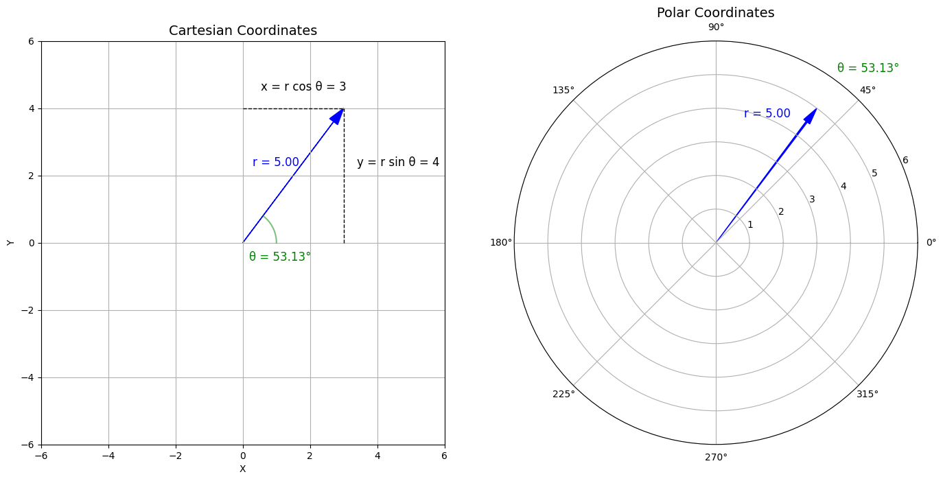
For the key idea of the algorithm, we need to understand how a point in the bivariate Cartesian coordinate system can be translated to polar coordinates. I’ve illustrated this in Figure 1:
In the bivariate Cartesian system (left subplot), we need the x and y coordinates to define the point $A$ $(3,4)$. Alternatively, we can describe this point using polar coordinates (right subplot): $A$ can be uniquely determined by its Euclidean distance $r=5$ from the origin (radius), and the angle $\theta \approx 53.13°$ between the radius vector and the positive x-axis. The relationship between these coordinate systems is given by:
$$x = r \cos(\theta), \quad y = r \sin(\theta).$$
Code
import numpy as np
import matplotlib.pyplot as plt

def cartesian_to_polar(x, y):

    r = np.sqrt(x**2 + y**2)
    theta = np.arctan2(y, x)
    return r, theta

def plot_vector_cartesian_polar(x, y):

    r, theta = cartesian_to_polar(x, y)

    # create a figure
    fig = plt.figure(figsize=(14, 6.5))

    #### left Subplot ####
    ax_cart = fig.add_subplot(1, 2, 1)
    limit = max(abs(x), abs(y), r) + 1
    ax_cart.set_xlim(-limit, limit)
    ax_cart.set_ylim(-limit, limit)

    # blue vector
    ax_cart.arrow(0, 0, x, y, head_width=0.3, head_length=0.5, fc='blue', ec='blue', length_includes_head=True)

    # projection lines
    ax_cart.plot([x, x], [0, y], 'k--', linewidth=1)
    ax_cart.plot([0, x], [y, y], 'k--', linewidth=1)

    # green arc for theta
    theta_range = np.linspace(0, theta, 100)
    arc_x = 1 * np.cos(theta_range)
    arc_y = 1 * np.sin(theta_range)
    ax_cart.plot(arc_x, arc_y, 'g-', alpha=0.5)

    # annotations
    ax_cart.annotate('x = r cos θ = 3', xy=(.25, 4.25), textcoords="offset points", xytext=(10,10), fontsize=12)
    ax_cart.annotate('y = r sin θ = 4', xy=(3.1, 2), textcoords="offset points", xytext=(10,10), fontsize=12)
    ax_cart.annotate(f'r = {r:.2f}', xy=(0, 2), textcoords="offset points", xytext=(10,10), fontsize=12, color='blue')
    ax_cart.annotate(f'θ = {np.degrees(theta):.2f}°', xy=(-.1, -.1), textcoords="offset points", xytext=(10, -15), fontsize=12, color='green')

    # labels and title
    ax_cart.set_title('Cartesian Coordinates', fontsize=14)
    ax_cart.set_xlabel('X')
    ax_cart.set_ylabel('Y')
    ax_cart.grid(True)
    ax_cart.set_aspect('equal')

    ##### right Subplot ####
    ax_polar = fig.add_subplot(1, 2, 2, projection='polar')

    # blue vector in polar coordinates
    ax_polar.arrow(theta, 0, 0, r,
                   width=0.01, head_width=0.05, head_length=0.5,
                   fc='blue', ec='blue', length_includes_head=True)

    # annotations
    ax_polar.annotate(f'r = {r:.2f}', xy=(np.pi * .45, 3.5),
                      textcoords="offset points", xytext=(10,10), fontsize=12, color='blue')
    ax_polar.annotate(f'θ = {np.degrees(theta):.2f}°', xy=(theta, r+1),
                      textcoords="offset points", xytext=(0, 10), fontsize=12, color='green')

    # title
    ax_polar.set_title('Polar Coordinates', fontsize=14)

    # r lim
    ax_polar.set_rlim(0, limit)

    # enable grid and labels
    ax_polar.grid(True)

    # layout adjustments
    plt.subplots_adjust(left=0.01, right=0.99, top=0.99, bottom=0.01, wspace=0.01)
    plt.show()


plot_vector_cartesian_polar(x = 3, y = 4)
What about Gaussians?
How does Figure 1 relate to bivariate Gaussian data? Remember that the desired probability density of $(X, Y)$ is $$ f_{X,Y}(x, y) = \frac{1}{2\pi} e^{-\frac{1}{2}(x^2 + y^2)}, $$ which is a radially symmetric distribution with respect to the origin. Using the trigonometry of Figure 1, we can define the bivariate Gaussian distribution using polar coordinates. This is a joint distribution of the r.v.s radius $R$ (the distance to the origin) and the angle $\Theta$ (between the point vector and the positive X axis). To derive the density for this joint distribution, we note that $R$ and $\Theta$ come from applying a transform $g(\cdot)$ to $X$ and $Y$:
$$ \begin{bmatrix}r\\ \theta\end{bmatrix} = g\begin{pmatrix}\begin{bmatrix}x\\ y\end{bmatrix} \end{pmatrix} := \begin{bmatrix}\sqrt{x^2 + y^2}\\ \tan^{-1}\left(\frac{y}{x}\right) \end{bmatrix}, \qquad r\geq0, \quad \theta\in[0,2\pi]. $$
The inverse transformation is
$$ \begin{align} \begin{bmatrix}x \\ y \end{bmatrix} = g^{-1}\begin{pmatrix}\begin{bmatrix}r\\ \theta\end{bmatrix}\end{pmatrix} := \begin{bmatrix} r \cdot \cos \theta \\ r \cdot \sin \theta \end{bmatrix}.\label{eq:transxy} \end{align} $$
The change of variables (CoV) formula gives the joint density of $[R \ \Theta]’$ as
$$ \begin{align} f_{R,\Theta}(r,\theta) =&\, f_{X,Y}\left(g^{-1}\left([r\ \theta]’\right)\right) \cdot \left\lvert \det\left[\frac{\mathrm{d}g^{-1}(\boldsymbol{z})}{\mathrm{d}\boldsymbol{z}}\Big\vert_{\boldsymbol{z} = [r\ \theta]’}\right] \right\rvert\notag\\ =&\, f_{X,Y}\left(g^{-1}\left([r\ \theta]’\right)\right) \cdot \lvert J\rvert,\label{eq:vtvcov} \end{align} $$
The Jacobian determinant $J$ for this CoV is computed as
$$ J = \det\begin{pmatrix} \frac{\partial x}{\partial r} & \frac{\partial x}{\partial \theta} \\ \frac{\partial y}{\partial r} & \frac{\partial y}{\partial \theta} \end{pmatrix}. $$
From the components in \eqref{eq:transxy} we get
$$ \begin{align*} \frac{\partial x}{\partial r} =&\, \cos\theta, \quad \frac{\partial x}{\partial \theta} = -r \sin\theta,\\ \frac{\partial y}{\partial r} =&\, \sin\theta, \quad \frac{\partial y}{\partial \theta} = r \cos\theta. \end{align*} $$
The Jacobian determinant hence becomes $$ \begin{align*} J =&\, \det\begin{pmatrix} \cos\theta & -r \sin\theta \\ \sin\theta & r \cos\theta \end{pmatrix}\\ =&\, \cos\theta \cdot r \cos\theta - \sin\theta \cdot (-r \sin\theta)\\ =&\, r \cdot (\cos^2\theta + \sin^2\theta)\\ =&\, r, \end{align*} $$ and so $|J| = r$. Substituting the expressions in \eqref{eq:vtvcov} obtains $$ \begin{align*} f_{R,\Theta}(r, \theta) =&\, \frac{1}{2\pi} r\exp\left(-\frac{1}{2}r^2\right)\\ =&\, f_\Theta(\theta) \cdot f_R(r) \end{align*} $$ where $$ \begin{align} f_\Theta(\theta) = \frac{1}{2\pi} \quad \textup{and} \quad f_R(r) = r \cdot \exp\left(-\frac{1}{2}r^2\right).\label{eq:rthetadens} \end{align} $$ Note that the independence of $\Theta$ and $R$ follows from the independence of $X$ and $Y$. Therefore, $f_{R, \Theta}(r, \theta)$ is simply the product of the marginal densities $f_R(r)$ and $f_\Theta(\theta)$.
Let’s look closer at the two densities in \eqref{eq:rthetadens}:
-
$f_\Theta(\theta)$ is the density of a uniformly distributed r.v. $\Theta$ on $[0,2\pi]$. This seems intuitive: $\theta$ is a randomly drawn angle, measured in radians.
-
$f_R(r)$ is the density of a Rayleigh distributed r.v. $R$ on $[0,\infty)$ with parameter $\sigma = 1$. This also makes intuitive sense: The probability of observing larger radii $r$ decreases exponentially, which matches our expectations for a bivariate normal distribution.
The Box-Muller Algorithm
The Box-Muller Transform elegantly converts uniform random variables to Gaussian ones: It uses samples from two independent standard uniform random variables, $U_1,\,U_2\sim U[0,1]$ to generate samples of $R$ and $\Theta$, cf. the distributions in \eqref{eq:rthetadens}. These samples are then transformed to independent Gaussian samples using of $g^{-1}(\cdot)$. Here’s the algorithm.
Algorithm: Box-Muller
- Sample $U_1, U_2 \sim U(0, 1)$.
- Obtain polar coordinates: $$ R = \sqrt{-2 \log U_1}, \quad \Theta = 2\pi U_2. $$
- Transform back to Cartesian coordinates: $$ X = R \cos \Theta, \quad Y = R \sin \Theta. $$
For step 2, it is straightforward to show that $$ \Theta = 2\pi U_2 \sim U[0,2\pi]. $$ Here’s why $R = \sqrt{-2 \log U_1}\sim \textup{Rayleigh}(\sigma=1)$:
The CDF of a $\textup{Rayleigh}(\sigma=1)$ r.v. $R$ is $F_R(z) = 1 - \exp(-z^2/2)$. We solve $F_{R}(z) = U_1$ for $z$, where $U_1 \sim \text{U}[0,1]$: $$ z = \sqrt{-2 \log(U)}. $$
We thus use inverse transform sampling to sample from $R$.
Python Implementation
Here’s how to implement the Box-Muller Transform in Python function:
import numpy as np

def box_muller_transform(n_samples):
    # step 1:
    U1 = np.random.uniform(0, 1, n_samples)
    U2 = np.random.uniform(0, 1, n_samples)

    # step 2:
    R = np.sqrt(-2 * np.log(U1))
    Theta = 2 * np.pi * U2

    # step 3:
    X = R * np.cos(Theta)
    Y = R * np.sin(Theta)

    return U1, U2, R, Theta, X, Y
Let’s generate some samples using box_muller_transform(). Note that the function not only outputs draws of $X$ and $Y$ but also draws of the uniform random variables $U_1$, $U_2$ and as well as draws of the polar coordinates $R$ and $\Theta$.
# generate samples
U1, U2, R, Theta, X, Y = box_muller_transform(n_samples = 2500)
Visualization
To inspect the outcomes, we create visualizations using matplotlib and seaborn. We arrange these plots in a grid layout.
import matplotlib.gridspec as gridspec

# subplots
fig = plt.figure(figsize=(12, 15))
gs = gridspec.GridSpec(3, 1, height_ratios=[1, 1, 1])

# plot uniform samples U1 vs U2
ax1 = fig.add_subplot(gs[0, 0])
ax1.scatter(U1, U2, alpha=0.3, edgecolor='none', s=10)
ax1.set_title('Uniform Samples (U₁ vs U₂)')
ax1.set_xlabel('U₁')
ax1.set_ylabel('U₂')
ax1.set_xlim(0, 1)
ax1.set_ylim(0, 1)
ax1.set_aspect('equal')

# R vs Theta in polar plot
ax2 = fig.add_subplot(gs[1, 0], projection='polar')
ax2.scatter(Theta, R, alpha=0.5, edgecolor='none', s=10)
ax2.set_title('Polar Coordinates (R vs Θ)', va='bottom')

# Gaussian samples X vs Y
ax3 = fig.add_subplot(gs[2, 0])
ax3.scatter(X, Y, alpha=0.3, edgecolor='none', s=10)
ax3.set_title('Gaussian Samples (X vs Y)')
ax3.set_xlabel('X')
ax3.set_ylabel('Y')
ax3.set_xlim(-5, 5)
ax3.set_ylim(-5, 5)
ax3.set_aspect('equal')
ax3.grid(True, which='both', linestyle='--', linewidth=0.5)

# adjust layout
plt.tight_layout()
plt.show()

Kernel density estimates of the marginal distributions of $X$ and $Y$ closely resemble the charactersitic bell shape.
import matplotlib.pyplot as plt
import seaborn as sns
import numpy as np
from scipy.stats import norm

# gaussian densities
x_vals = np.linspace(-4, 4, 1000)
gaussian_dens = norm.pdf(x_vals)

plt.figure(figsize=(10, 7))

# KDE X
plt.subplot(1, 2, 1)
plt.plot(
    x_vals, gaussian_dens,
    color='red', linestyle='--', label='Standard Gaussian'
)
sns.kdeplot(X, color='blue', label='KDE')
plt.title("KDE of X")

# KDE Y
plt.subplot(1, 2, 2)
plt.plot(
    x_vals, gaussian_dens,
    color='red', linestyle='--', label='Standard Gaussian'
)
sns.kdeplot(Y, color='blue', label='KDE')
plt.title("KDE of Y")

# legend
handles, labels = plt.gca().get_legend_handles_labels()
fig = plt.gcf()
fig.legend(handles, labels, loc='lower center', ncol=2, frameon=False)

plt.tight_layout(rect=[0, 0.1, 1, 1])

plt.show()

… and that’s it for now!